The perceptron is the Illiad of neural nets, a predecessor that all following ML literature is built on, and just like Homers Illiad it is an anachronism of its time. 1957 by Frank Rosenblatt created, by his own account, "the first machine which is capable of having an original idea". Just like many other revolutionary ideas it would take about a generation for Rosenblatts ideas to really come into fruition.
Rosenblatts core idea was to identify the smallest component of the human brain, the neuron, and simulate it in a computer program. Then, if you have 86 billion copies of this computer program (as many neuron as in a human brain) all connected with each other you should be able to build an artificial human brain, a modern day Frankenstein.
So how do we do this? First of all we need to create a model of the neuron that we can express as an algorithm. A neuron is probably the most specialized cell in the human body. It has dendrites, axons, synapses, neurotransmitters, ion channels, etc. etc. But a simple model of the neuron looks something like this:
Synaptic receptors receive a neurotransmitter which lead to a synaptic current that creates a change in membrane potential. If the potential across all the synapses crosses a threshold the neuron has an action potential which will send neurotransmitters to a neighbouring neuron.
We can formalize this model of a neuron using mathematical expressions:
$$ z = f(\boldsymbol{x}) = \sum_{i=1}^{n}{w_ix_i} + b = \boldsymbol{w}^T\boldsymbol{x} + b $$
$$ g(\boldsymbol{z}) = \begin{cases} 1, && \text{if } z \gt 0 \\ 0, && \text{otherwise} \end{cases} $$
$$ y = g(f(\boldsymbol{x})) $$
What we're doing is taking a weighted sum of inputs $\boldsymbol{w}^T\boldsymbol{x}$ plus a bias and if that sum exceeds 0 the neuron fires (outputs 1). This is the mathematical model of what Rosenblatt called the *perceptron*. The point of it is that it maps onto the functions of an individual neuron as close as mathematically possible.
By adjusting the weights and the bias of the perceptron we can "teach" it to classify inputs into a binary target label. Formally, we do this by minimizing a loss $\mathcal{L}$ across a set of examples.
$$ \boldsymbol{w}^*, b^* = \text{argmin}_{w,b} \frac{1}{N} \sum_{i=1}^N \mathcal{L}(\boldsymbol{w}^Tx^{(i)} + b, y^{(i)}) $$
So, using some input data that maps a set of inputs into a set of binary outputs we can find a set of weights that classifies inputs as either 0 (perceptron not active) or one (perceptron active). The process of finding these weights is what we call learning (as in machine learning). A natural question now becomes, what should $\mathcal{L}$ be? Rosenblatt created what's called the perceptron learning algorithm, which has been replaced by more efficient algorithms. In the perceptron learning algorithm we calculate the weighted sum to get a prediction, $\gamma_{predicted}$ and compare it with a target, $\gamma_{target}$ to get an error value $\text{error} = \gamma_{target} - \gamma_{predicted}$ this error is then used to update weights using:
$$ dw_i = lr \cdot \text{error} \cdot w_i $$
$$ w_i = w_i + dw_i $$
We can demonstrate the perceptron learning by generating some random x, y pairs and then applying a label to the data based on some rule, as an example i'll choose $R = x > y \text{ then } 1 \text{ otherwise } 0$. R can be any operation on the two variables, the point is that the perceptron can learn any rule that outputs 0 or 1 linearly. The goal of the perceptron will then be to learn this rule by updating the weights so that $w_1x + w_2y = \text{target}$ where target is determined by the rule.
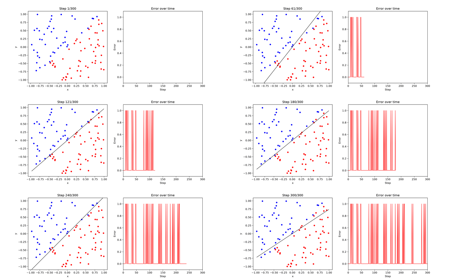
The line generated is defined by $w_1x + w_2y$ which is also known as the decision boundary.
This is all it takes to create the simples neural net! What we have, demonstrated in fig1, is a computer learning a rule by observing data from it's environment. The perceptron can be written in about 100 lines of C++ and is seen as a trivial programming example for basically anyone but a novice. The original perceptron was programmed using punch cards by Rosenblatt in 1957 on an IBM 704, the first computer to handle floating point numbers and described by IBM as "high-speed electronic calculator".
While a single neuron can learn any binary rule the artificial brain should contain billions of these.
If one perceptron can learn a single linear rule will a network of many perceptron allow you to model nonlinear relationships? The answer is yes. A network of perceptrons, a *neural network* can perform any continuous input-output mapping. The proof of this is known as the universal approximation theorem and provides the mathematical foundation for the applicability of neural networks in practise. The caveat here is that Rosenblatts learning algorithm falls apart here. In order for our single perceptron to be able to learn a rule it needs to have a datapoint that it can compare to in order to calculate an error, this is only available for the last layer in the network. We need another way to train the perceptrons deeper into the the network by propagating the errors back through all of the layers for them to be able to update their weights accordingly. This is where the concept of backpropagation and gradient-based learning algorithms come in.
Backpropagation adjusts the weights of each neuron in the network by taking the derivative of each parameter with respect to the loss. This is in contrast with the perceptron learning algorithm where we just calculated the error and let that error guide us to an approximate solution. This is a nice and simple solution for a 2D linear problem, but if we have more dimensions and hidden layers in our network it doesn't yield useful results since we only get information about the output and have no way of informing other layers about the error. Using the chain rule we know that:
$$ \frac{\partial{J}}{\partial{\theta_1}} = \frac{\partial{J}}{\partial{x_L}}\frac{\partial{x_L}}{\partial{x_{L-1}}}...\frac{\partial{x_3}}{\partial{x_2}}\frac{\partial{x_2}}{\partial{x_1}}\frac{\partial{x_1}}{\partial{\theta_1}} $$
$$ \frac{\partial{J}}{\partial{\theta_2}} = \frac{\partial{J}}{\partial{x_L}}\frac{\partial{x_L}}{\partial{x_{L-1}}}...\frac{\partial{x_3}}{\partial{x_2}}\frac{\partial{x_2}}{\partial{\theta_2}} $$
You can see that most of the terms used to calculate $\frac{\partial{J}}{\partial{\theta_2}}$ are identical to $\frac{\partial{J}}{\partial{\theta_1}}$ which means that we can calculate the derivatives we need by just doing one forward pass. We now get a simple formula for calculating the gradient with respect to the parameters
$$ \frac{\partial{J}}{\partial{\theta}} = g_{out}L^{\theta} $$
Computing $L$ is an entirely local process which we get by computing the derivative of its functional form, $f'$ which is then evaluated at the *operating point* $[x_{in}, \theta]$ to obtain $L = f'(x_{in}, \theta)$. To compute $g_l$ (the series of partial derivaties) we need to know $g_{l+1}$ and so we have a recursive relation defined by
$$ g_{in} = g_{out}L^x $$
This recursive relation is the essence of backprop and allows us to send error signals from the output layer to every parameter in the network.
The full backpropagation algorithm consists of a forward pass which provides a loss and a backward pass which provides all the gradients we need to calculate the derivative of the loss with respect to each parameter.
With backpropagation defined we can go on to construct our network. Remember that our single perceptron model only learned linear functional relationships, its hypothesis space was defined by all linear functions (like $y = ax + b$). We know from the universal approximation theory that a neural net can learn any functional relationship by staking neurons into layers and then letting layers feed into each other. I demonstrate this by constructing a neural net with 2 inputs, one hidden layer with 4 neurons and 1 output neuron and letting it learn the XOR function which is a simple nonlinear function that our previous single perceptron network would not be able to learn.
By the way the XOR problem is famous in the deep learning community since it was used to prove that perceptrons were incapable of learning nonlinear relationships back in 1969 by Marvin Minsky. The (very real) problems that Minsky identified were only fixed by adding a hidden layer and introducing the backpropagation algorithm in the 1980s.
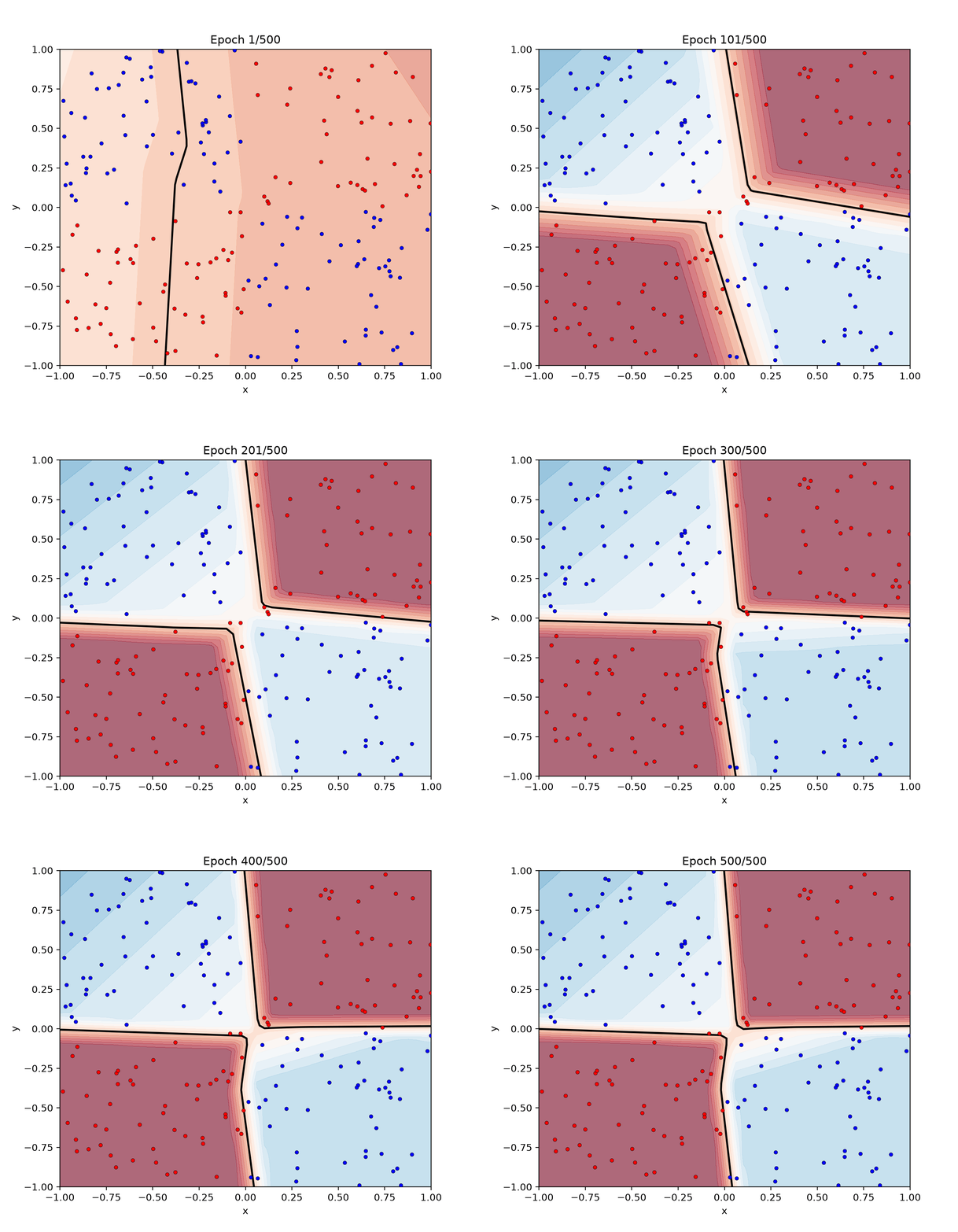
From the figure you'll see the resulting decision boundary (black lines), the output of the network for each $(x, y)$ pair (shown as colors from red to blue), the target values of each point (shown either as a red or a blue dot) animated over 500 epochs.
Rosenblatt never got to see his invention materialize into real artificial intelligence. The algorithms we use today that power recommendation engines, image generators and LLMs are all based on his models. More importantly the universal approximation theorem tells us that *any* signal can be approximated and predicted using a neural network a truly groundbreaking result that lets us ponder what neural nets *can't* do rather than what they can do. The story of the perceptron is the story of human ingenuity and incremental progress, ironically a very human one.